Isoline plots on triangle meshes in Matlab
Alec Jacobson
March 09, 2012
I recently posted how to plot nice looking iso intervals of scalar fields on triangle meshes using matlab. Along with the intervals I gave an ad hoc way of also showing isolines. This works ok if your data has fairly uniform gradient but they're not really isolines.
Here's a little matlab function to output real isolines. Save it in a file called isoline.m:
function [LS,LD,I] = isolines(V,F,S,iso)
  % ISOLINES compute a list of isolines for a scalar field S defined on the
  % mesh (V,F)
  %
  % [LS,LD,I] = isolines(V,F,S,iso)
  %
  % Inputs:
  %   V  #V by dim list of vertex positions
  %   F  #F by 3 list of triangle indices
  %   S  #V list of scalar values defined on V
  %   iso #iso list of iso values
  % Outputs:
  %   LS  #L by dim list of isoline start positions
  %   LD  #L by dim list of isoline destination positions
  %   I  #L list of indices into iso revealing corresponding iso value
  %
  % alternative: tracing isolines should result in smaller plot data (every
  % vertex only appears once
  %

  % make sure iso is a ROW vector
  iso = iso(:)';
  % number of isolines
  niso = numel(iso);

  % number of domain positions
  n = size(V,1);
  % number of dimensions
  dim = size(V,2);

  % number of faces
  m = size(F,1);

  % Rename for convenience
  S1 = S(F(:,1),:);
  S2 = S(F(:,2),:);
  S3 = S(F(:,3),:);

  % t12(i,j) reveals parameter t where isovalue j falls on the line from
  % corner 1 to corner 2 of face i
  t12 = bsxfun(@rdivide,bsxfun(@minus,iso,S1),S2-S1);
  t23 = bsxfun(@rdivide,bsxfun(@minus,iso,S2),S3-S2);
  t31 = bsxfun(@rdivide,bsxfun(@minus,iso,S3),S1-S3);

  % replace values outside [0,1] with NaNs
  t12( (t12<-eps)|(t12>(1+eps)) ) = NaN;
  t23( (t23<-eps)|(t23>(1+eps)) ) = NaN;
  t31( (t31<-eps)|(t31>(1+eps)) ) = NaN;

  % masks for line "parallel" to 12
  l12 = ~isnan(t23) & ~isnan(t31);
  l23 = ~isnan(t31) & ~isnan(t12);
  l31 = ~isnan(t12) & ~isnan(t23);

  % find non-zeros (lines) from t23 to t31
  [F12,I12,~] = find(l12);
  [F23,I23,~] = find(l23);
  [F31,I31,~] = find(l31);
  % indices directly into t23 and t31 corresponding to F12 and I12
  %ti12 = sub2ind(size(l12),F12,I12);
  %ti23 = sub2ind(size(l23),F23,I23);
  %ti31 = sub2ind(size(l31),F31,I31);
  % faster sub2ind
  ti12 = F12+(I12-1)*size(l12,1);
  ti23 = F23+(I23-1)*size(l23,1);
  ti31 = F31+(I31-1)*size(l31,1);

  % compute actual position values
  LS = [ ...
    ... % average of vertex positions between 2 and 3
    bsxfun(@times,1-t23(ti12), V(F(F12,2),:)) + ...
    bsxfun(@times,  t23(ti12), V(F(F12,3),:)) ...
    ; ... % average of vertex positions between 2 and 3
    bsxfun(@times,1-t31(ti23), V(F(F23,3),:)) + ...
    bsxfun(@times,  t31(ti23), V(F(F23,1),:)) ...
    ;... % average of vertex positions between 2 and 3
    bsxfun(@times,1-t12(ti31), V(F(F31,1),:)) + ...
    bsxfun(@times,  t12(ti31), V(F(F31,2),:)) ...
    ];
  LD = [...
    ... % hcat with average of vertex positions between 3 and 1
    bsxfun(@times,1-t31(ti12), V(F(F12,3),:)) + ...
    bsxfun(@times,  t31(ti12), V(F(F12,1),:)) ...
    ;... % hcat with average of vertex positions between 3 and 1
    bsxfun(@times,1-t12(ti23), V(F(F23,1),:)) + ...
    bsxfun(@times,  t12(ti23), V(F(F23,2),:)) ...
    ;... % hcat with average of vertex positions between 3 and 1
    bsxfun(@times,1-t23(ti31), V(F(F31,2),:)) + ...
    bsxfun(@times,  t23(ti31), V(F(F31,3),:)) ...
    ];

  % I is just concatenation of each I12
  I = [I12;I23;I31];

end
Then if you have a mesh in (V,F) and so scalar data in S. You can display isolines using:
colormap(jet(nin));
trisurf(F,V(:,1),V(:,2),V(:,3),'CData',S,'FaceColor','interp','FaceLighting','phong','EdgeColor','none');
axis equal;
[LS,LD,I] = isolines(V,F,S,linspace(min(S),max(S),nin+1));
hold on;
plot([LS(:,1) LD(:,1)]',[LS(:,2) LD(:,2)]','k','LineWidth',3);
hold off
set(gcf, 'Color', [1,1,1]);
set(gca, 'visible', 'off');
%O = outline(F);
%hold on;
%plot([V(O(:,1),1) V(O(:,2),1)]',[V(O(:,1),2) V(O(:,2),2)]','-k','LineWidth',2);
%hold off
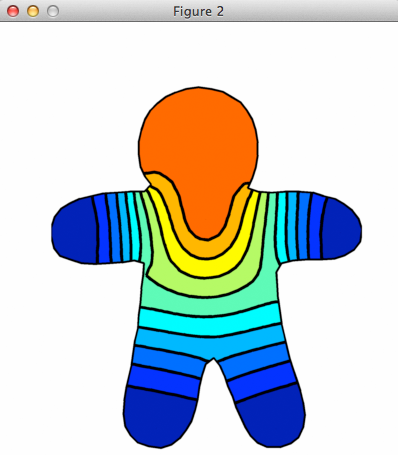
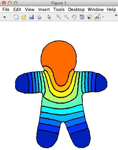
Uncomment the last lines to display the outline of the mesh. This produces:
If you use the my anti-alias script you can get pretty good results, almost good enough for a camera-ready paper: