Deriving the probability density function of a non-uniform sampling of the circle

Alec Jacobson

May 19, 2013

weblog/

I recently posted about non-uniformly sampling a sphere and visualizing the result. As I was examining the result, I though it would be more convenient just to derive the probability density function analytically. This is an exercise in transforming the probability density function of one random variable into that of another. As a warmup I followed this systematic approach on math.stackexchange for a 2d problem of non-uniformly sampling a circle, actually just the first quarter of the circle. The scheme under consideration is to first sample x and y from the unit square uniformly, then normalize (x,y) to unit length and read off the angle θ. This transformation of normalizing then converting to polar angle, takes these two uniformly samples to a non-uniform sampling of the quarter circle, θ in [0,π/2). In other words the probability density functions of the first variables x and y are both 1 for x,y in [0,1) and we'd like to know what the probability density function of θ is. We begin by acknowledging that for any reasonable function u we have the equality: E(u(θ)) = ∬ u(θ) 1_0≤x<11_0≤y<1 dxdy. Now let's define θ = atan2(y/sqrt(x²+y²),x/sqrt(x²+y²)) = atan2(y,x). Here we'll perform a change of variables. Let y = t and let x = t/tan θ. This means that dxdy = dx/dθ dθ dy/dt dt = -t/sin²(θ) dθdt, hence: E(u(θ)) = ∬ u(θ) 1_{0≤t/tan θ<1}1_0≤t<1 -t/sin²(θ) dθdt We also know that for every reasonable function u that: E(u(θ)) = ∬ u(θ) f_Θ(θ) dθ, where f_{Θ(θ) is the (so far unknown) probability density function of our random variable Θ. Setting this equal to the equation above we have:

f_Θ(θ) = ∫ 1_{0≤t/tan θ<1}1_0≤t<1 -t/sin²(θ) dt.

So far we've been dealing with indefinite integrals, but we can convert to a definite one by evaluating the 1 functions, leaving:

f_Θ(θ) = ∫₀^{min(1,tan θ)} -t/sin²(θ) dt
= -1/sin²(θ) ∫₀^{min(1,tan θ)} t dt
= -1/sin²(θ) · min(1,tan θ)²/2

Finally we can also write this as a piecewise function:

f_Θ(θ) = { 1/cos²θ/2 θ≤π/4
1/sin²θ/2 θ>π/4

We can verify this with the following small matlab program:
sam = 4000000;
method = 'naive';
%method = 'uniform';
switch method
case 'naive'
N = normalizerow(rand(sam,2));
case 'uniform'
S = rand(sam,1)*pi/2;
N = [cos(S(:,1)) sin(S(:,1))];
end
S = atan2(N(:,2),N(:,1));

% analytic solution
f = @(th) (th<pi/4).*(1/cos(th).^2) + (th>=pi/4).*(1/sin(th).^2);

[h,b] = hist(S,100);
% normalize so integral is 1
h = h./sum(h*(pi/2/numel(b)))
bar(b,h);
hold on;
plot(th,-f(th),'LineWidth',2);
hold off

which produces:

Actually, it's also pretty straight forward to derive the probability density function geometrically rather than analytically.

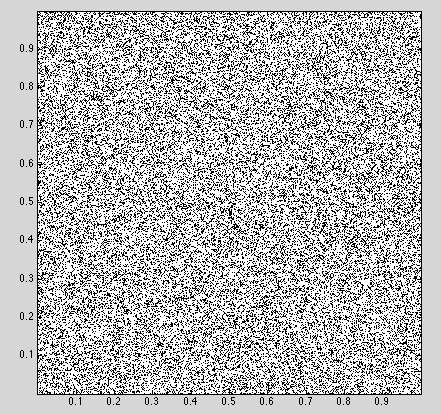
Start with our uniform sampling of the unit square:

When we project this sampling to the quarter circle (green), we're really integrating along each ray (blue) of angle θ (grey):

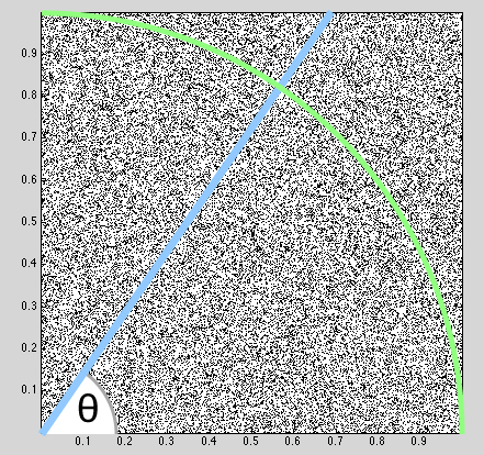
If we had only considered the points inside the circle then we would indeed have a uniform sampling as this integral is then independent of θ. This invites a scheme called rejection sampling: choose x,y in the unit cube but only keep those inside the circle.

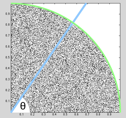
It's the points that lie outside the circle that cause this kind of sampling to be biased, non-uniform.

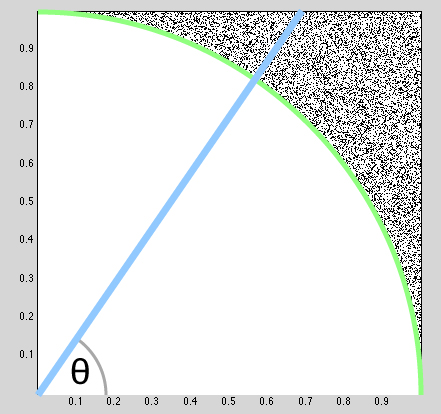
We can compute the integral along this ray geometrically. Since the sampling is uniform, it amounts to just computing the length of the line segment. We just need to know for a given angle θ where the ray intersects the unit square.

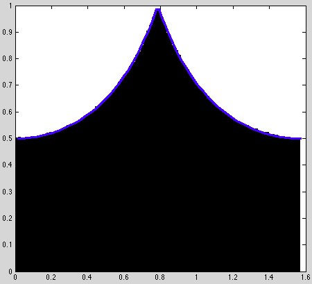
First let's consider θ≤π/4. We know that x = 1 and by the polar coordinations we have that y = r cosθ, thus the radius and the length of these line segments are 1/cos θ. Likewise for θ>π/4 we have line segments of length 1/sin θ. These values are the length of the line segments, and since we're integrating a uniform density function, they're also the mass accumulated along the line segment. Finally we must account for the change in units, exchanging each small change in angle with a change in area. Namely by exactly this length divided by two (two because the thin space between two close rays is a triangular, rather than rectangular). Thus, by multiplying our mass by this change we have:

f_Θ(θ) = {
(1/cos²θ)/2

(1/sin²θ)/2
θ≤π/4
θ>π/4,

which matches the analytic result above.

Update: I'm not so confident that this derivation geometric derivation tells the whole story anymore.}