Mosek, a commercial solver, writes in its documentation that it's often advantageous to convert a separable quadratic program:
min_x 1/2 |Fx - c|^2
subject to Ax <= b
with x a n-long vector, into a conic program of the form
min_{x,t,y} y - x'F'c
subject to  Ax <= b
and         Fx - t = 0
and         2y >= t't
introducing t as a new vector variable and y as a new scalar variable.
It's rather straightforward to verify that these two problems are equivalent. But what's the intuition behind it?
To understand this, we'll need to be comfortable with two ways of visualizing an energy function: as a line plot or height-field surface and viewed from above as a topographic map of isolines.
Recall that an energy function E(x) is just a scalar function of one or more variables in the vector x. To be sure, this means E(x) takes in a list of numbers in x and spits out a single number.
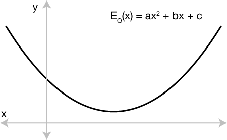
In our original quadratic program, the energy was a quadratic function of x. If x were a only a single variable (scalar) then we can rewrite 1/2 |Fx - c|^2 as f^2/2 x^2 - 2fc x + c^2. This is simply a quadratic function x, familiar after substitution as: ax^2 + bx + c. We know that plotting this will reveal a parabola:
Minimizing E(x) in this picture means walking along values of x and tracing the curve until reaching the vertex, the point with minimal E(x) and, notably, zero derivative.
Conceptually when we convert this simpler 1D quadratic problem E(x) = ax^2 + bx + c into a conic program we introduce a new variable y. It's important that we really recognize y as a variable. So far we don't know its value. If we stopped here we'd have an optimization problem:
min_{x,y} ax^2 + bx + c
where y spans an infinite null space of solutions: the energy only measures the effect of x; any choice of y is OK.
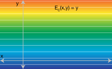
But here comes the trick, we place y directly in the objective function: E_C(x,y) = y. This new energy is linear in only y. If we know plot it as a topographical map over the xy-plane we see a function decreasing indefinitely in the downward direction:
Obviously if we stop here and minimize over x and y, we could get any value of x and we'll simply get y=-∞. The final step is to add a conic constraint on y according to the original quadratic function of x. Namely we ask that y >= ax^2 + bx + c: y should be above the original quadratic function. Since we're only working with scalar x and scalar y we can plot the feasible region as on the xy-plane. y must be above the red region:
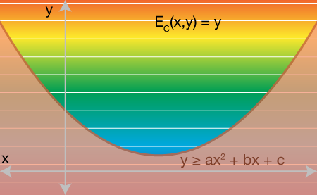
Now we can imagine minimizing y by traveling downward, we'll eventually hit the red region's wall. Since we have full freedom to move in the x direction, too, we can continue downward only if we slide along the wall toward the minimum of the original quadratic function E(x).
Higher dimensions: This scenario is significantly easier to visualize for the 1d problem. However, the intuition extends to higher dimensions. If x is a vector then E(x) is a hyper-paraboloid over x. When we introduce y, we still just add a single new orthogonal dimension. Then minimizing the value of y we'll smash into this hyper-paraboloid and slide toward the minimum.
Solvers: This explanation is meant to give some intuition as to why this conversion works. It's not meant as a explanation of how interior-point conic programming solvers work. I also do not explain why it's sometimes more efficient to convert least squares quadratic programs to conic programs. Admittedly the conditions for a successful conversion in terms of efficiency still allude me.