There are different flavors of the multigrid method. Let's consider the geometric subclass and within that the "Galerkin" or projection-style multigrid method. This method is favorable because it only requires discretization at the finest level and prolongation and restriction between levels. This means, given a problem A1 x1 = B1 on the finest mesh, we don't need to know how to create an analogous problem A2 x2 = B2 on the second finest mesh and so on. Instead, we define A2 = R A1 P where R is the #coarse vertices by #fine vertices restriction operator taking fine mesh values to coarse mesh values and P is the #fine vertices by #coarse vertices prolongation operator. A Galerkin multigrid V-cycle looks something like this:
x1 according to A1 x1 = B1r1 = B1 - A1 x1r2 = R r1A2 = R A1 PA2 u2 = r2u1 = P u2, x1 += u1 x1 according to A1 x1 = B1Often (for good reasons), we take the restriction operator to be the transpose of the prolongation operator R = P'. When we're working with nested meshes, it's natural to use the linear interpolation operator as P.
This V-cycle if A1 x1 = B1 is coming from a quadratic energy minimization problem:
min  ½ x1' A1 x1 - x1' B1
 x1
Suppose we freeze our current guess x1 and look for the best update u1, we'd change the problem to
min  ½ (x1 + u1)' A1 (x1 + u1) - (x1+u1)' B1
 u1
Rearranging terms according to u1 this is
min  ½ u1' A1 u1 - u1' (B1 - A1 x1) + constants
 u1
Now we recognize our residual r1 = B1 - A1 x1. Let's substitute that in:
min  ½ u1' A1 u1 - u1' r1
 u1
If we were to optimize this for u1 we'd get a system of equations:
A1 u1 = r1
Instead, let's make use of our multires hierarchy. The coarse mesh spans a smaller space of functions that the finer mesh. We can take any function living on the coarse mesh u2 and interpolate it to give us a function on the fine mesh u1 = P u2, thus we could consider restricting the optimization search space of u1 functions to those we can create via P u2:
min  ½ (P u2)' A1 (P u2) - (P u2)' r1
 u2
rearranging terms and substituting R = P' we get:
min  ½ u2' R A1 P u2 - u2' R r1
 u2
finally optimizing this for u2 we get a system of equations:
R A1 P u2 = R r1
or
A2 u2 = r2
This Galerkin-style multigrid is great because we don't need to worry about re-discretizing the system matrix (e.g. using FEM on the coarse mesh) or worry about redefining boundary conditions on the coarse mesh. The projection takes care of everything.
But there's a catch.
For regular grids with carefully chosen decimation patterns (#vertices on a side is a power of 2 plus 1) then the projection matrix will be well behaved. Each row corresponding to a fine mesh vertex will at most 1 vertex if perfectly align atop a coarse mesh vertex and will involve the nearest 2 vertices on the coarse mesh if lying on a coarse mesh edge. Then examining a row of A2 = P' A1 P we can read off the change in the stencil. Let's say A1 is a one-ring Laplacian on the fine mesh. Hitting it on the left with P' will form the matrix P' A1, a row of which corresponds to a coarse mesh vertex and the columns to the fine mesh vertices it "touches". Since coarse vertices lie exactly at fine mesh vertices, this will simply connect each coarse mesh to its "half-radius-one-ring", i.e. the fine mesh vertices lying on coarse mesh edges around it. Finally hitting this matrix with P on the right creates A2 = P' A1 P connecting coarse to coarse vertices. Since each coarse vertex was connected to its "half-radius-one-ring" via the fine mesh, now in P' A P` all coarse mesh vertices are connected to its true one-ring neighbors: just like if we built the Laplacian directly on the coarse mesh. The sparsity pattern is maintained.
For irregular grids this is unfortunately not the case. Each row in P will contain, in general, d+1 entries. When we examine P' A1, we see that we smear the stencil around the coarse mesh to include the "half-radius-one-rings" from d+1 nearest fine-mesh vertices. This effect is repeated when finally creating P' A1 P. We see the sparsity worsening with each level.
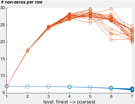
Here's a plot of the number non-zeros per row of the projected system matrix for a multires hierarchy with 7 levels.
The orange lines shows the average number of non-zeros per row for the cotangent Laplacian projected down different sequences of random irregular meshes of the unit square. You can see a rough 2x increase in the number of non-zeros in the beginning and then things taper-off as the meshes get very coarse: meshes range from roughly 2562 to 42. The blue lines show the average number of non-zeros per row for the cotangent Laplacian rediscretized (aka rebuilt from scratch) on each mesh: this is and should be roughly 7 for any triangle mesh (the slight decrease is due to the increase effect of the boundary on the average).
This doesn't look so bad. Even for the third level (562 vertices) the number of non-zeros per row is 25: still _very sparse).
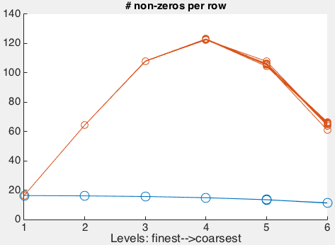
Things get worse, much worse in 3D.
Already the average number of non-zeros per row of a the 3D tet-mesh Laplacian is not neatly bounded to 7, though it tends to be around 16 for a "reasonable mesh".

In this plot we see the number of non-zeros in the projected system matrix increasing by around a factor of 3 each level, peaking around 112 on the 173 mesh. Notice on the 93=729 vertex grid the average number of non-zeros is 100. That's a sparsity ratio of 13% or 729,000 non-zeros: not very sparse for such a small mesh. Especially considering that the rediscretization system matrix would have 12 non-zeros per row, a sparsity ratio of 1.6%, or only 8,700 total non-zeros.
I didn't have the patience to let this run on a larger initial fine-mesh, but you can imagine that the situation gets drastically worse. Galerkin multigrid fails to improve performance and gets choked by memory consumption on irregular 3D tetrahedral meshes using piecewise linear prolongation operators.
$E = mc^2$