Consider a triangle mesh with $n$ vertices and $m$ faces. If we store a piecewise linear function $u$ as a vector of values at each vertex, $u \in \mathbb{R}^n$, then we can define the Laplacian matrix $L \in \mathbb{R}^{n \times n}$ as discretizing the Dirichlet energy: $$ u^T L u = \frac{1}{2} \sum_{f \in F} \int_{\Omega_f} \|\nabla u\|^2 \, dx $$ where $\nabla u$ is the gradient of $u$. This results in the _usual_ cotangent Laplacian, whose properties are by now well understood and appreciated.
Given this Laplacian $L$, we can model problems like smoothing, for example, given some possibly noisy function $v$, again a piecewise linear function with values at each vertex, we can solve the minimization problem: $$ \min_u \frac{1}{2}(u - v)^T M (u - v) - \lambda \frac{1}{2} u^T L u $$ where $M \in \mathbb{R}^{n \times n}$ is a diagonal "mass matrix," accounting for triangle areas around each vertex.
Since this is a convex quadratic minimization problem, we can solve it using linear algebra. The solution is $$ u = \underbrace{(M + \lambda L)^{-1} M}_{\text{vertex-based smoothing operator}} v. $$
But sometimes my noisy function is defined as a (piecewise-constant) function $V$ with values at each face, $V \in \mathbb{R}^m$, and I'd like as output a similar per-face function $U \in \mathbb{R}^m$ which is smoothed proportional to my parameter $\lambda$.
I'm particularly interested in having good smoothing behavior even when the mesh is coarse and/or has non-uniform resolution.
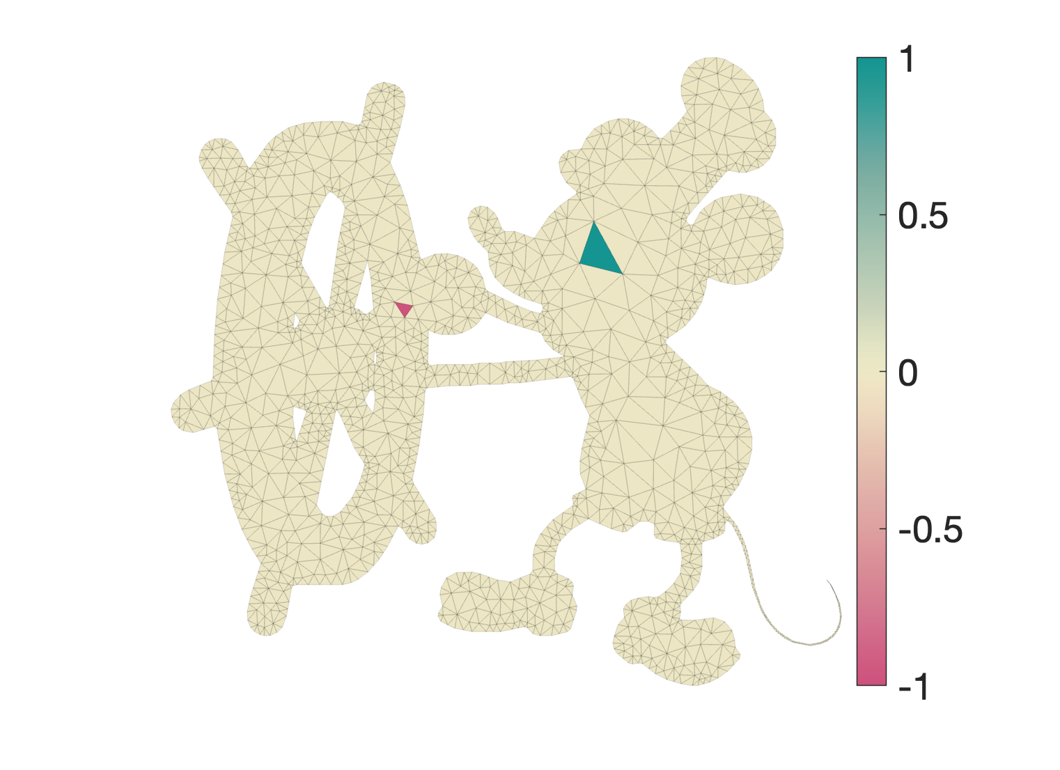
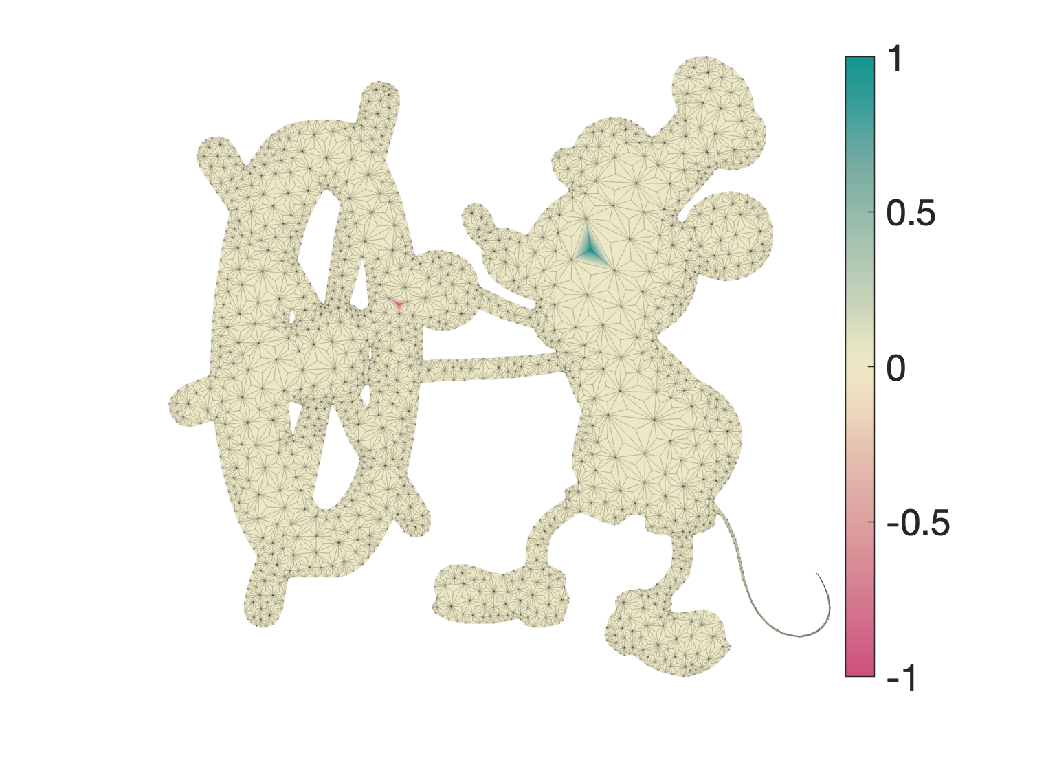
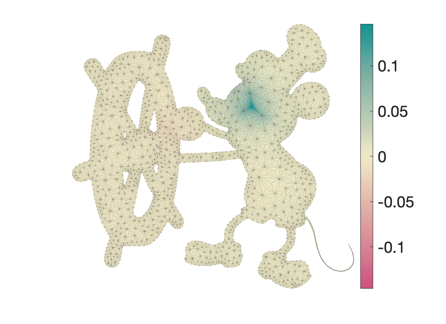
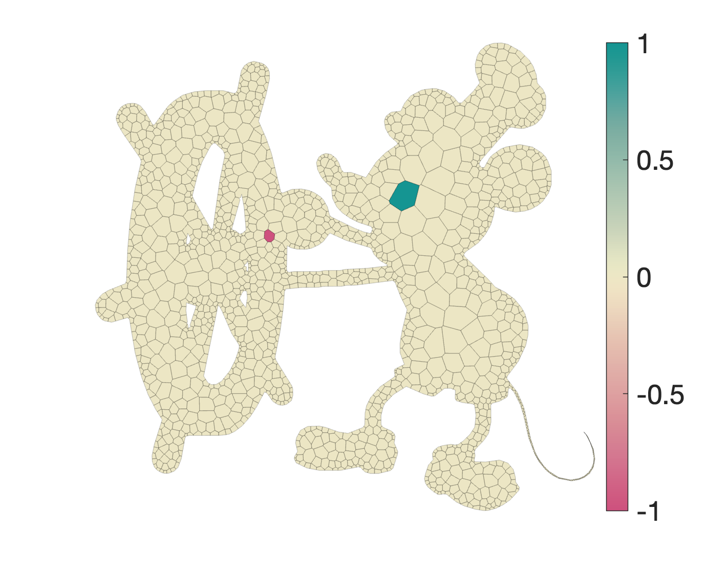
As a running example consider this Mickey Mouse domain with a +1 and -1 scattered in a field of 0 values per-element.
Similar to computing per-verex normals for shading, we could use an area-weighted average of face values on to vertex values: $v = W V$ where $W \in \mathbb{R}^{n \times m}$ where $ W_{if} = A_f / \sum_{g \in \text{faces}(i)} A_g$ if face $f$ is incident on vertex $i$ and $W_{if} = 0$ otherwise.
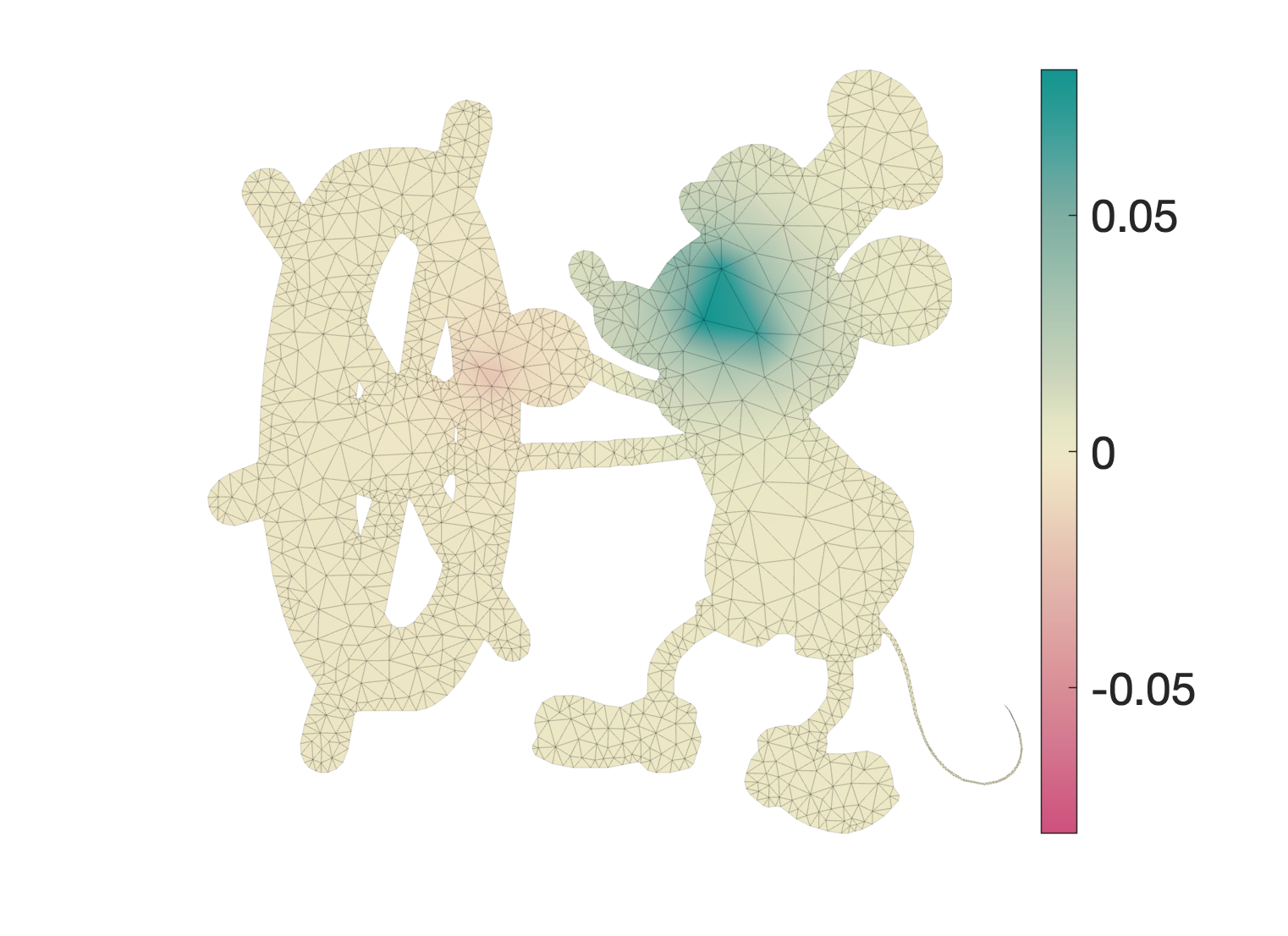
Now we can apply the vertex-based smoothing operator above to smooth these vertex values. For $\lambda = 1000$ this is looking reasonable; notice the colorbar continues to rescale.
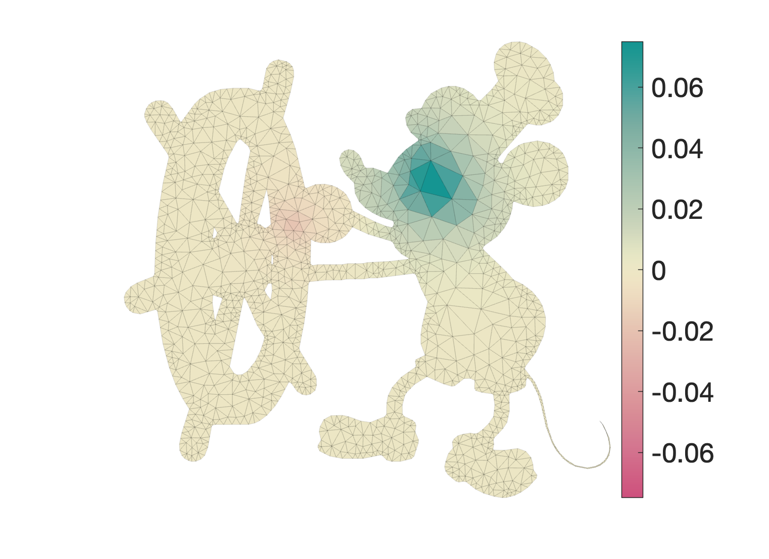
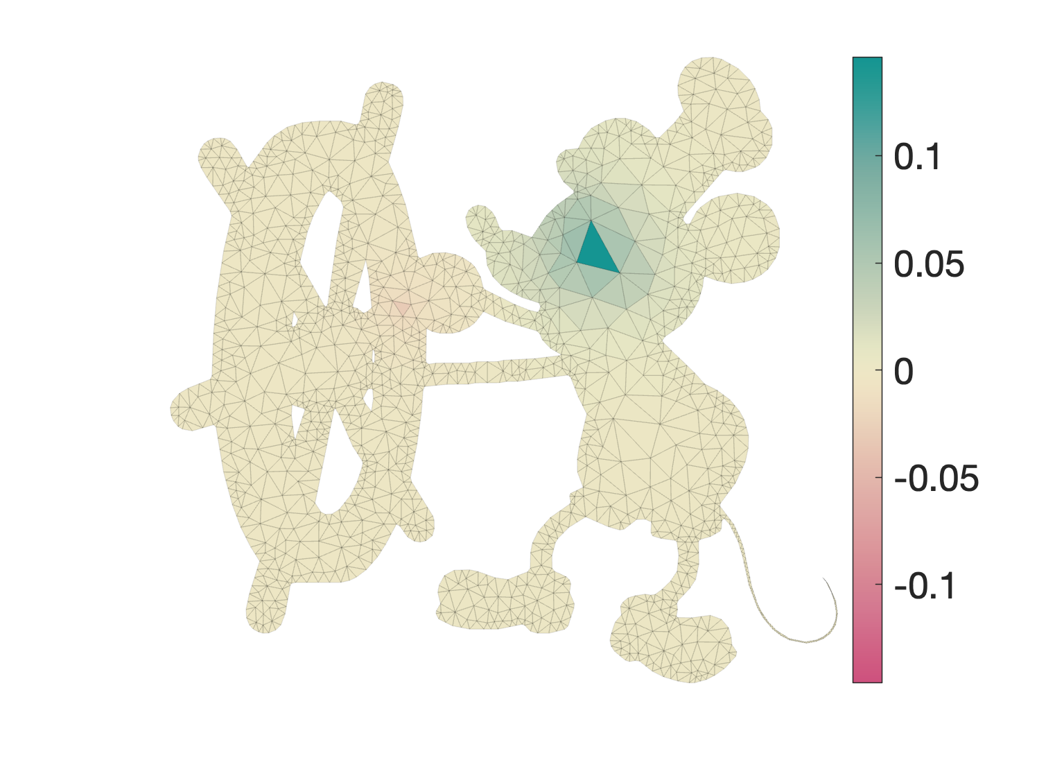
Finally to get back onto faces, we could use a uniformly-weighted average of vertex values onto face values: $U = N u$ where $N \in \mathbb{R}^{m \times n}$ where $N_{fi} = 1/3$. Composing all the steps our candidate element-based smoothing operator can be defined as: $$ U = \underbrace{N (M + \lambda L)^{-1} M W}_{\text{naive element-based smoothing operator}} V $$ For this large $\lambda=1000$ example this looks alright.
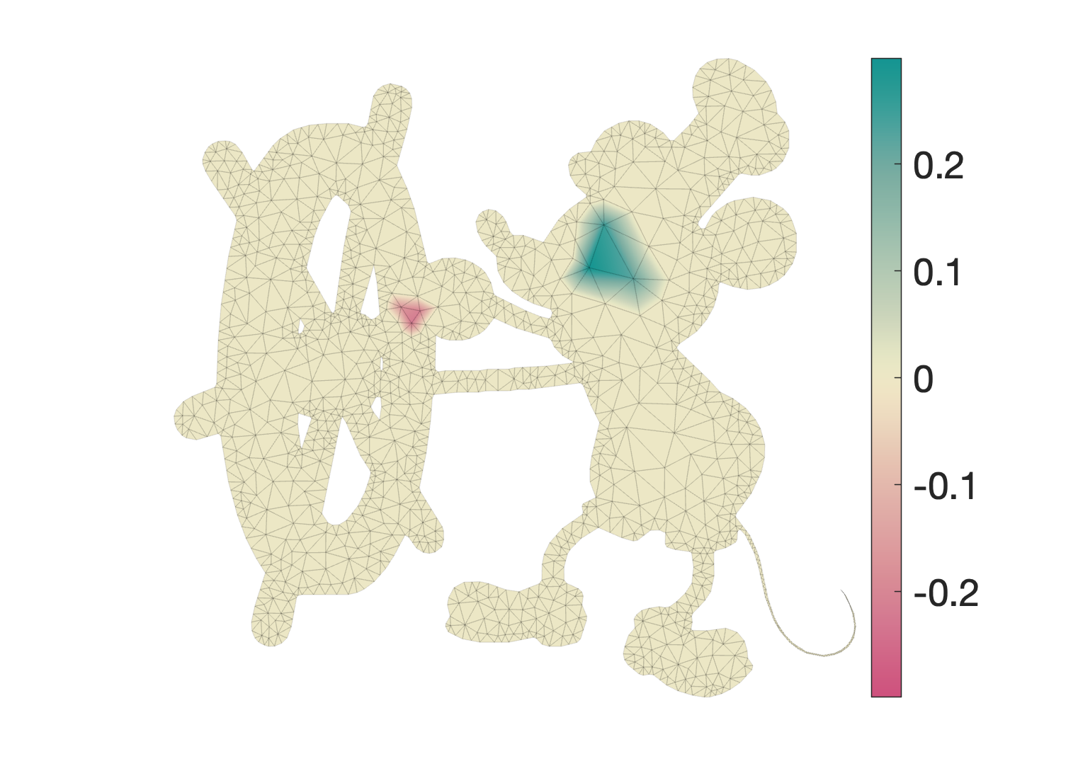
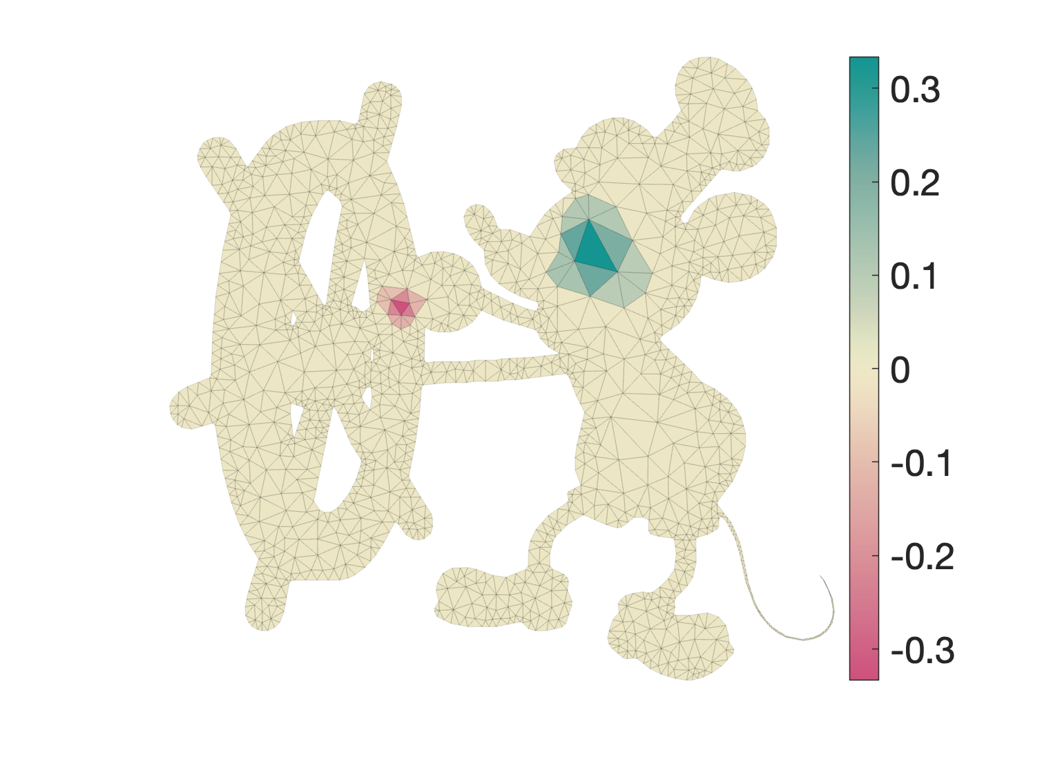
But what happens if we set $\lambda=0$? In this case, any reasonable smoothing operator should act like the identity, i.e. $U = V$. In this case we'd compute: $$ U = N W V. $$ There's no reason for $N$ and $W$ to annihilate each other, and indeed in our example we see that values are smeared to one-ring neighbors:
Moreover, this operation is not conservative. That is, the integral of output values over the domain is not the same as the integrated input: \begin{align} \int_{\Omega} U \, dx &\neq \int_{\Omega} V \, dx \\ \sum_{g \in \text{faces}} A_g U_g &\neq \sum_{f \in \text{faces}} A_f V_f \\ 529.699 & \neq 426.717 \text{ (for this example).} \end{align}
So then let's try to layout some criteria for what makes a good element-based smoothing operator: $$ U = \underbrace{Q_\lambda}_{\text{element-based smoothing operator}} V $$
The implied element-based Laplacian should also, in turn, have the properties discussed in "Discrete Laplace operators: No free lunch" [Wardetzky et al. 2007]:
To construct an element-based smoothing operator, first build the so-called false barycentric subdivision of the input mesh by inserting one vertex at the barycenter of each triangle, splitting each triangle into three smaller ones. This results in a mesh with $n+m$ vertices and $3m$ faces. Build the operator $S = [0\ \ I] \in \mathbb{R}^{(n+m) \times m}$ which trivially copies values from per-element data to the "barycenter-vertices" f this subdivided mesh. Visualizing $S V$ on our running example looks like:
Now, let's pull a trick. Instead of building the usual mass matrix on this mesh. Let's build one that has zeros for all the old vertices and original triangle areas for these new barycenter-vertices: $\tilde{M} \in \mathbb{R}^{(n+m) \times (n+m)}$ where $\tilde{M}_{n+f,n+f} = A_f$ and $\tilde{M}_{i,j} = 0$ otherwise. Build a cotangent Laplacian matrix $\tilde{L} \in \mathbb{R}^{(n+m) \times (n+m)}$ in the usual way on this mesh. Then we can do vertex-based smoothing using these matrices: $$ \tilde{u} = (\tilde{M} + \lambda \tilde{L})^{-1} \tilde{M} S V, $$ which produces the following result for $\lambda=1000$:
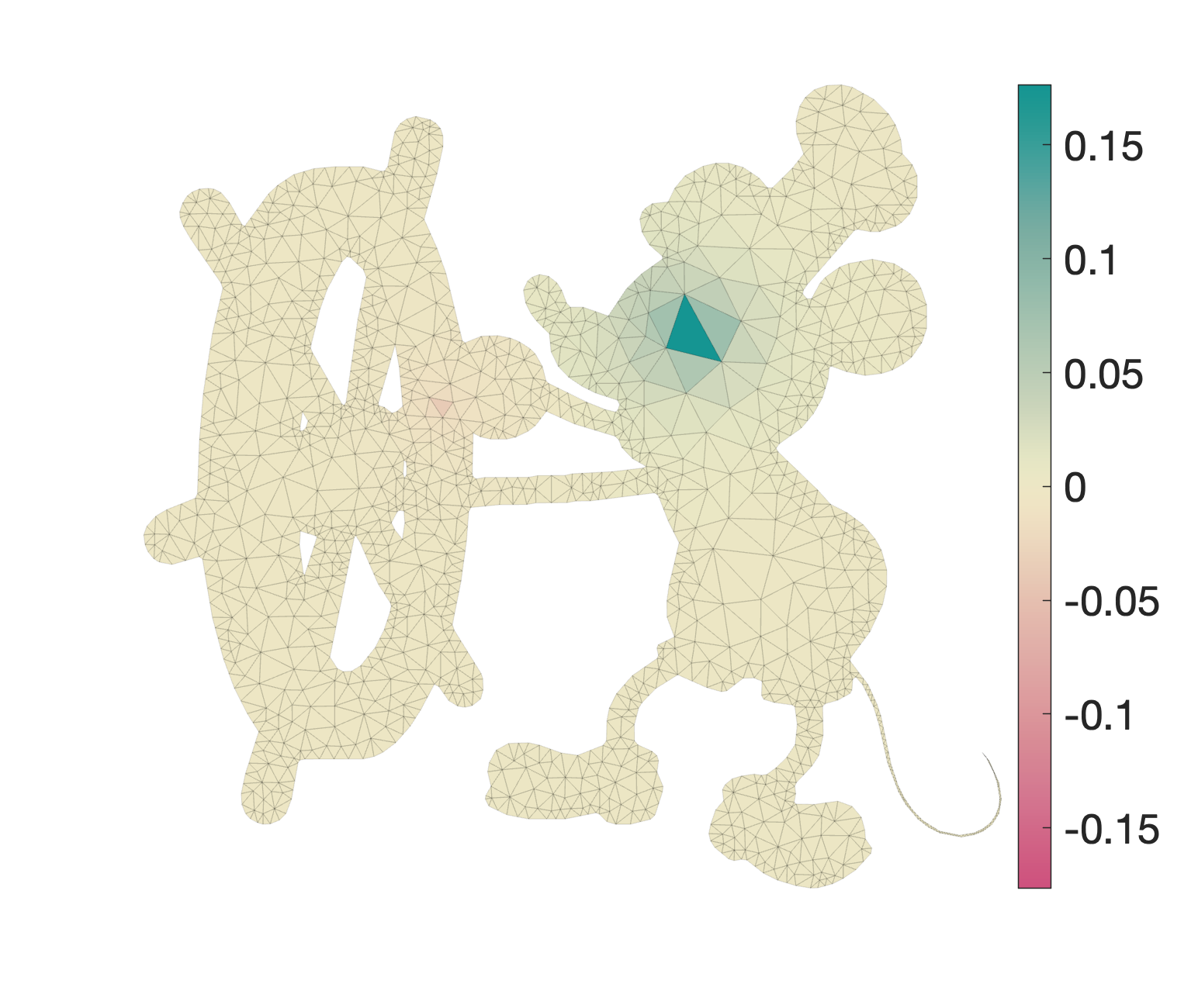
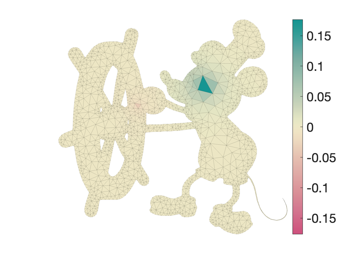
Finally, use the transpose of $S$ to pull these values back onto the original mesh: $$ U = \underbrace{S^T (\tilde{M} + \lambda \tilde{L})^{-1} \tilde{M} S}_\text{element-based smoothing operator} V, $$ which produces the following result for $\lambda=1000$:
We can do a slight rearrangement by substituting $\tilde{M} S = S A$ where $A \in \mathbb{R}^{m \times m}$ is a diagonal matrix with the original triangle areas on the diagonal. Then we can write the element-based smoothing operator as: $$ U = \underbrace{S^T (\tilde{M} + \lambda \tilde{L})^{-1} S}_{H_\lambda} A V, $$ where please don't manifest the dense matrix $H \in \mathbb{R}^{m \times m}$, but conduct actions (like multiplication) against it using the decomposition above.
So, what are we using as the Laplacian here? Let's consider the limit of $\lambda \rightarrow \infty$ or rather let's divide the original energy minimization above by $\lambda$ so that we can consider: $$ L_\text{element} = H^{-1} = \lim_{\lambda \rightarrow 0} \left(S^T \left( \frac{1}{\lambda} \tilde{M} + \tilde{L}\right)^{-1} S\right)^{-1} $$
My interpretation of this is that we're using the usual Laplacian on the false-barycentric subdivision and then "picking out" the behavior of its inverse at the face-vertices. This is very different than picking out before inverting $S^T \tilde{L} S$, as that would result in a trivial diagonal matrix.
My assesment of the properties above is:
The "local support" property of this Laplacian is questionable. If we care about local support because derivatives are local and so their graph discretizations should be local (why?), then this one clearly is not. If we care about local support because we want to be able to solve large systems by exploiting sparse matrices, then we achieved that.
The "linear precision" property seems similarly questionable. The $\tilde{L}$ is linearly precise $V$ is peicewise constant so it can't really represent a linear function. We could sample a linear function at triangle barycenters and then $S V$ would be a very non-linear function (with zeros at all original vertices). So in this sense it is not linearly precise. I'm not sure if linear precision in the sense of Wardetzky et al. --- who motivate this property with vector-valued applications --- matters for scalar-field smoothing.
From a finite-element perspective, the false-baricentric subdivision is a scary mesh: all the original corners angles got cut in half, and there's a increase in vertex valences. So instead of using FEM to build the Laplacian, we can build the intrinsic Delaunay Laplacian on the false-barycentric subdivision mesh to improve numerics:
While we're flipping edges, an even simpler approach in the planar case is to use sqrt3-subdivision connectivity rules: flip all original interior edges. Before applying the final $S^T$ we get this solution visualized over the subdivided mesh:

That mesh looks far less scary from a finite-element perspective. And here's the
result back on the original faces:
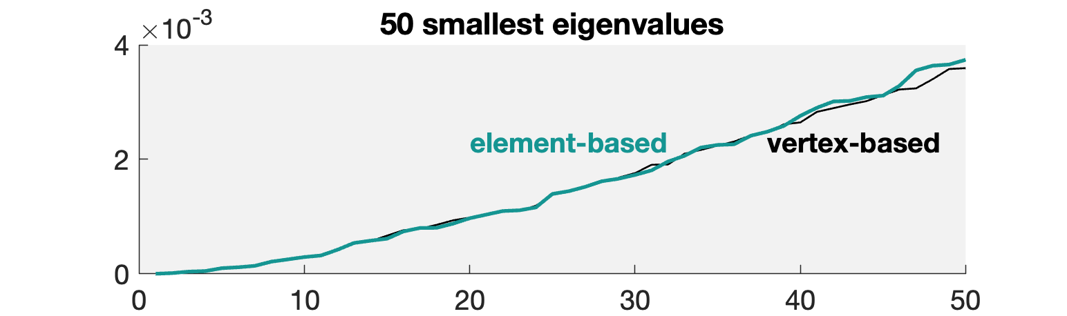
I leave convergence analysis for future work, but I'm hopeful after some quick tests that this isn't much worse than convergence of the usual pieceswise linear discretization. The spectrum already looks pretty good on the running example.
Nick Sharp pointed out that since a Laplacian implies a notion of mean curvature, this construction should imply a per-face discrete mean curvature. One way to do this is to apply a small amount ($\lambda = 10^{-8}$) of smoothing to the face barycenters in 3D:
$$ -\Delta X = H \hat{n} \approx \left(X - S^T (\tilde{M} + \lambda \tilde{L})^{-1} \tilde{M} S X\right)/\lambda $$Then I could recover the mean curvature $H$ by dotting with the unit face normals. Here's how that looks on a 3D mesh:
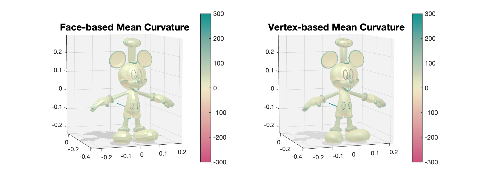
Compared to per-vertex discrete mean curvature computed using dihedral angles, the values are in the right ballpark.
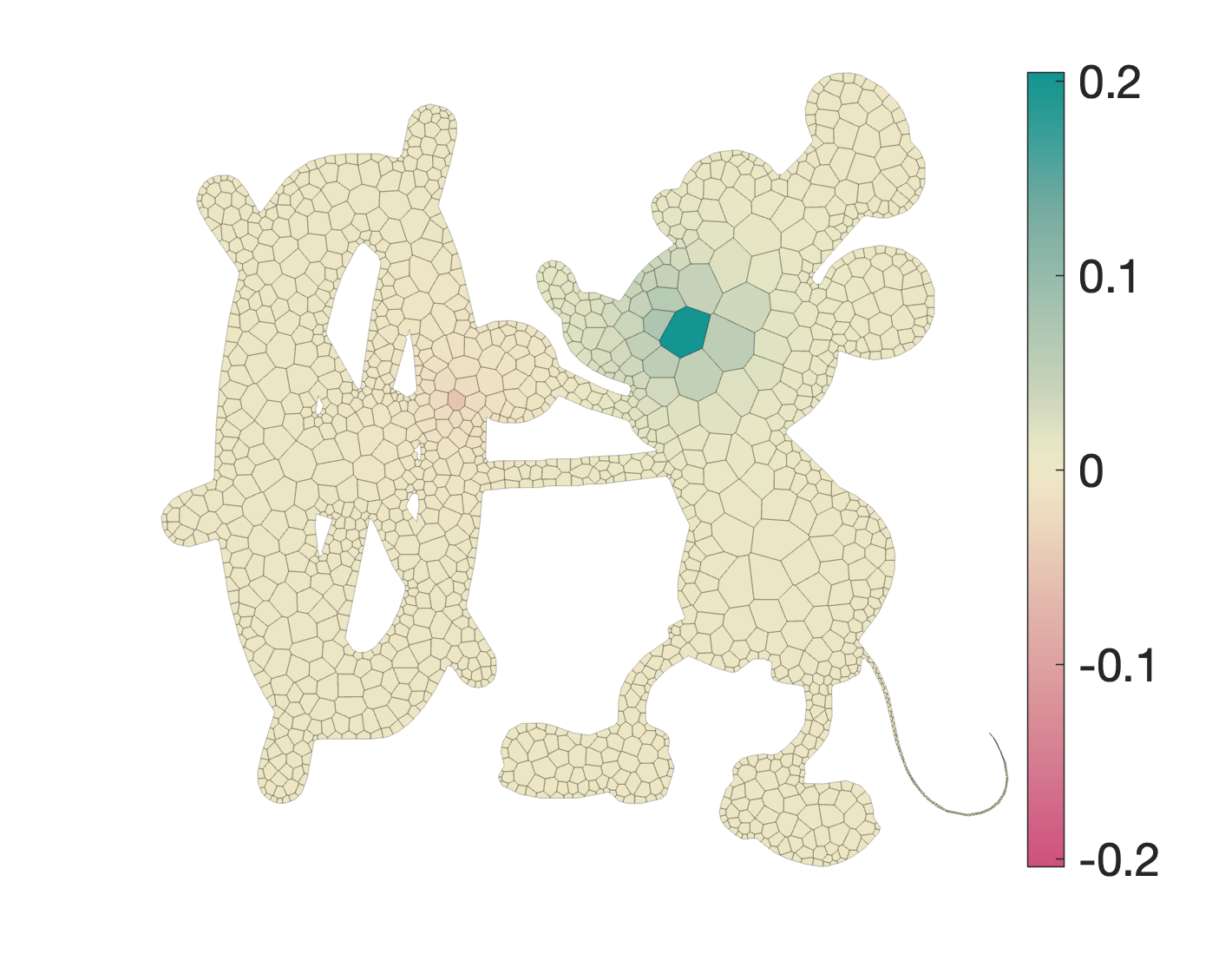
Nick also pointed out that this construction should work for polygon faces as well. Consider this polygon mesh analogous to our running example:
Following [Bunge et al.], we can subdivide each (star-shaped) polygon face by constructing a fan of triangles connected to a new vertex placed to minimize these triangles' squared areas. Then following everything as above, we get a satisfying smoothing: